#011 DS&A - Sorting - Omar ElKhatib

Sorting Techniques

Insertion sort algorithm and analysis

Insertion-sort(A)
{
    for j = 2 to A.length
        key = A[j]
        // insert A[j] into sorted sequence A[1...j-1]
        i = j-1
        while(i>0 and A[i] > key)
            A[i+1] = A[i]
            i = i-1
        A[i+1] = key
}

every time you visit an element you check the one before it if it's greater swap them , if their is a swap you compare the new element with old elements in array.

Worst case is Teta(n^2) is if the sorted list is backward sorted from biggest to lowest , and best case is Omega(n) if array is already sorted , and space complexity is O(1) called inplace which mean we don't use extra spaces.

We can't optimize it if we apply binary searching the comparison between new element and old elements is O(log n) and movement required is O(n) , in doubly linked list it require O(n) for comparison and O(1) for movement. In both cases we have bottleneck to O(n)

Merge sort algorithm and analysis

MERGE(A, p , q , r)
{
    n1 = q-p+1
    n2 = r-q
    let L[1...n+1] and R[1 to n2+1] be the new arrays
    for(i=1 to n1)
        l[i] = A[p+i-1]
    for(j=1 to n2)
        R[j] = A[q+j]
    L[n1+1] = inf
    R[n2+1] = inf
    i = 1 , j = 1
    for(k = p to r)
        if(L[i] <= R[j])
            A[k] = L[i]
            i=i+1
        else
            A[k] = R[j]
            j=j+1
}
// A is array , p is start index , q is end of sorted arr1 index , r is last index

The merge here work having a main array contain 2 sorted arrays inside of it

0	1	2	3	4	5	6	7
1	5	7	8	2	4	6	9

this will be divided into 2 arrays L and R

L from p to q

0	1	2	3	4
1	5	7	8	Inf

R from q+1 to r

0	1	2	3	4
2	4	6	9	Inf

after dividing the main array to 2 it will start to compare R[j] with L[i] if will increment the index of the lower like if L[i] < R[j]

i will be incremented by 1 , and inserting them into array , and note that Inf here is large number with same type of data.

then array will become

0	1	2	3	4	5	6	7
1	2	4	5	6	7	8	9

this algorithm will take O(n) for dividing arrays and n+n to copy elements back to array is O(n) so time taken is O(n)

space complexity is O(n) also.

merge-sort(A, p , r) - T(n)
{
    if p<r
        q=L[(p+r)/2]
        merge-sort(A,p,q) - T(n/2)
        merge-sort(A,q+1,r) - T(n/2)
        merge(A,p,q,r) - O(n)
}

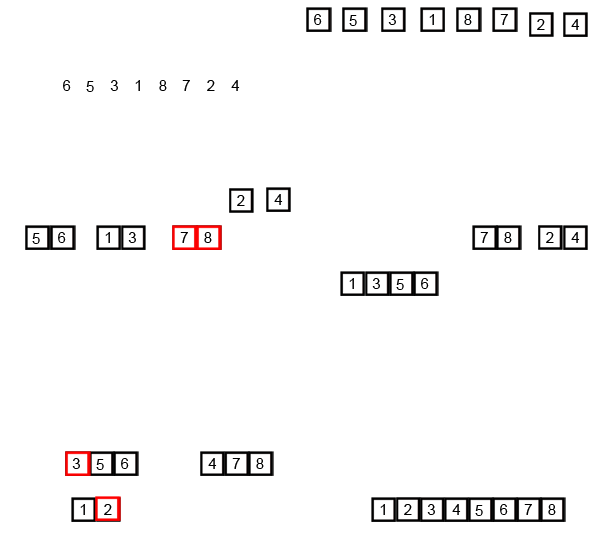
the size of stack required for merge-sort is log(n)+1 so space complexity is o(log n) and merge will require is O(n) so total is O(n) + O(log n) which n is dominated so O(n) is space complexity.

T(n) = 2*T(n/2)+O(n) = O(n*log(n) we use here the master theorem to calculate time complexity

so what ever is the size of problem it will always take O(n*log(n))

Quick sort algorithm and analysis

PARTITION(A,p,r)
{
    x = A[r]
    i = p-1
    for(j=p to r-1)
    {
        if(A[j] <= x)
        {
            i=i+1
            exchange A[i] with A[j]
        }
    }
    exhange A[i+1] with A[r]
    return i+1
}

Partition algorithm is about putting the last element of array in it's right place where left of it are values which less (no sorted) of it's value and right is greater (not sorted) . Since the for will loop
n times so time complexity will be O(n)

QUICKSORT(A,p,r) - T(n)
{
    if(p<r)
    {
        q = PARTITION(A,p,r) - O(n)
        QUICKSORT(A,p,q-1) - T(n/2)
        QUICKSORT(A,q+1,r) - T(n/2)
    }
}

Sorting quicksort anim.gif

it will keep sub-Quick-sorting and return every time it will face
p==r or
p>r

worst space complexity is O(n) and average is O(log n)

time complexity is T(n)=2*T(n/2)+O(n) = Teta(n log(n) ) using the master theorem

the worst case is where the number the last element is in the right order.

time complexity will be

T(n) = T(n-1) + O(n)
     = T(n-1)+cn
     = T(n-2)+c*(n-1)+c*n
     = T(n-3)+c*(n-2)+c(n-1)+c*n
     ...
     = c+2c+3c+...+c*n
     = O(n^2)

Introduction to heaps

heap trees are is a binary tree or 3-ary tree or n-ary tree.

let's talk about binary tree heap only , heap have their root is max heap and all nodes sub-tree should be smaller than the parent node.

A complete Binary tree of height h has 2h-1 nodes. Out of these 2h-1 are leaf nodes and rest (2h-1-1 are non-leaf)

complete binary tree

complete binary tree_1

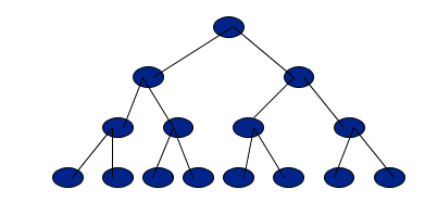
Canonical labeling of nodes

Label the Nodes in the level-wise fashion from left to right, as shown below: canonically labeled The advantage of canonical labeling is that such a tree can be stored in an array where value of a node is stored at the index equal to its label in the tree. Binary heap This way we will save a lot of memory because we do not need to store all the pointers. If you have noticed, there is a relationship between the labels of a node and its children above: Binary heap_1

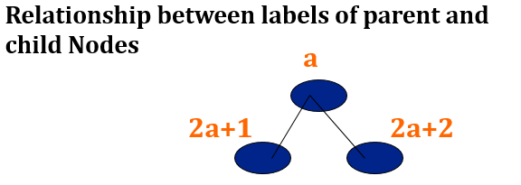
2*a is nothing but left shifting , so it's easy to implement in computer. 10 is a binary number represent 2 in decimal if i left shift it it will become 100 which is 4 in decimal.

This way, it becomes easy to move in either upward or downward direction of a tree, even when it is stored in an array.

almost complete binary tree

Below trees are NOT almost complete binary trees (the labeling has no meaning, because there are gaps). NOT almost complete binary tree

-- source

The input of an Algorithm affect the time complexity a lot let's take those cases

	insert	search	find min	delete
unsorted array	O(1)	O(n)	O(n)	O(n)
sorted array	O(n)	O(log n)	O(1)	O(n)
unsorted linked list	O(1)	O(n)	O(n)	O(n+1)=O(n)
min heap	O(log n)		O(1)	O(log n)

Max heapify algorithm and complete binary tree

to build A heap in first place we should re-arrange it in a way that the parent always bigger than children.

max-HEAPIFY(A,i)
{
    l = 2*i;
    r = 2*i+1;
    largest = i;
    
    if(l <= A.heap-size and A[i] > A[i]) largest = l; // check if it's have a left child 
    if(r <= A.heap-size and A[r] > A[largest]) largest = r; // check if it's have a right child
    if(largest != i)
    {
        exchane A[i] with A[largest]
        max-HEAPIFY(A,largest)
    }
}

the heart of this Algorithm is if we have sub-trees are max-heap but we need to make the root max-heap also.

time complexity is O(log n) which is the height of the tree , space complexity is the number of recursive calls O(log n)

Build max heap algorithm and analysis

BUILD-max-heap(A)
{
    A.heap-size = A.length
    for( i = floor(A.length/2) down to 1) 
        max-HEAPIFY(A,i)
}

take this array A as an example 9,6,5,0,8,2,1,3

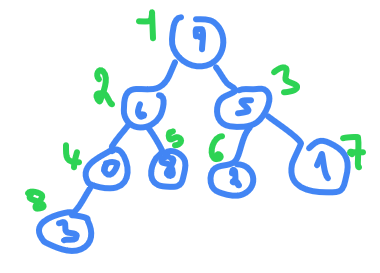
length of A is 8 floor(8/2)+1 = 4+1 = 5 (we add 1 because we start from 1 not 0)

so from index 5 to 1 we need to apply max-HEAPIFY(A,i) , index 5 is already a leaf so nothing to do go to index 4 0<8 so swap them

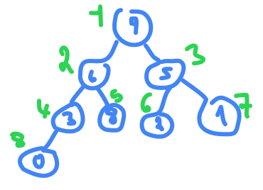
then in index 3 we have 5 > 2 > 1 so nothing to do , go to index 2 we have 6<8 so swap

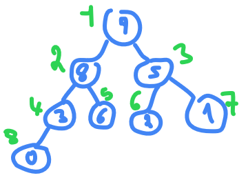
and index 1 is already the biggest so nothing to do.

what is the total time taking to build this max-HEAP ?

height of tree is log n and we are applying it n times so you will think that will take O(n log n) but it's not the time complexity is not the way to do it.

the number of nodes at height $h$ is $\leq {\frac {2^{\lfloor \log n\rfloor }}{2^{h}}}\leq {\frac {n}{2^{h}}}$

Therefore, the cost of heapifying all subtrees is:

${\begin{aligned}\sum _{h=0}^{\lfloor \log n\rfloor }{\frac {n}{2^{h}}}O(h)&=O\left(n\sum _{h=0}^{\lfloor \log n\rfloor }{\frac {h}{2^{h}}}\right)&=O\left(n\sum _{h=0}^{\infty }{\frac {h}{2^{h}}}\right)&=O(n)\end{aligned}}$

where is nothing than 2 (there is a proof for this)

and for space complexity required will be O(log n)

Extract max from heap

Heap-extract-max()
{
    if A.heap-size < 1
        error "heap underflow"
    max = A[1]
    A[1] = A[A.heap-size]
    A.heap-size = A.heap-size - 1
    max-HEAPIFY(A,1)
    return max
}

Now that we have the Heapify procedure, the Extract-Max procedure isn't hard to define at all. Suppose we have the following heap.

Extracting the node with maximum value is easy enough - by the definition of a heap, it is at the top. So we return it. Fine. Now the question is how to turn what remains,

back into a heap. We can almost run the heapify procedure on the whole thing, except that we have two complete binary trees, not one.

So we move the node at the bottom right to the top.

Now we can perform the Heapify procedure on the whole tree.

time taking is O(log n) and same for space.

Heap - increase key

Heap-Increase-Key(A, i, key)
// Input: A: an array representing a heap, i: an array index, key: a new key greater than A[i]
// Output: A still representing a heap where the key of A[i] was increased to key
// Running Time: O(log n) where n =heap-size[A]
1 if key < A[i]
2   error(“New key must be larger than current key”)
3 A[i] ← key
4 while i > 1 and A[Parent(i)] < A[i]
5   exchange A[i] and A[Parent(i)]
6   i ← Parent(i)

because it's increase a key we don't need from our key to be less than element so we return error, and we loop until we reach the root , and for every node we see it's parent if it's less or bigger than the key we exchange it.

if we need to decrease a node we need to max-heapify for the tree in that node , which in worst case will take O(log n)

Heap Sort

HEAP-sort(A)
{
    BUILD-max-HEAP(A)
    for(i = A.length down to 2)
    {
        exchange A[1] with A[i]
        A.heap-size = A.heap-size-1
        max-HEAPIFY(A,1)
    }   
}

we are running max-HEAPIFY n times so time complexity is O(n * log(n)) where log n is time complexity of max-HEAPIFY

Bubble sort

BubleSort(int a[] , n)
{
    int swapped,i,j;
    for(i=0;i<n;i++) {
        swapped = 0;
        for(j=0 ; j<n ; j++) {
            if(a[j] < a[j+1]){
                swap(a[j] , a[j+1]);
                swapped = 1;
            }
        }
        if(swapped == 0) break;
    }
}

Bubble sort algorithm

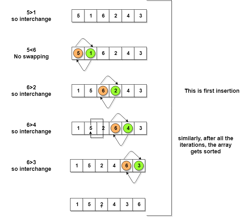
the worst case is reversed sorted array which is O(n^2)

and average case is O(k*n) and best case is O(n)

Bucket sort

bucket sort generally use to solve kind of problem where numbers are float and range from a to b with a and b are float.

0.35 , 0.12 , 0.43 , 0.15 , 0.04 , 0.50 , 0.132

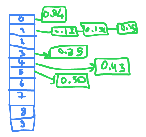
it will take first number . and put it in it's place if is already an element there it will sort them then printing them in order.

0.04 , 0.12 , 0.132 , 0.15 , 0.35 , 0.43 , 0.50

in best case where the numbers will be inserted without need to sort to place new item in cell so every insertion will take O(1) , so all the insertion will take O(n) and space complexity will be O(n+k)

the worst case O( (n/k) * n ) = O(n^2)

Counting sort

Counting sort have restrictions to apply , the restriction is that the input is in a range.

let's say our range is from 1 to 5

so we will take an array of 5 elements 2 2 3 4 1 5 1 5

INDEX	appearance
1	2
2	2
3	1
4	1
5	2

then we print them in order 1 1 2 2 3 4 5 5

time complexity is O(n+k) and space complexity is O(k)

the disadvantage we can not go outside range and if the range is big , and the elements are few

1 1000 2 3 so the amount of space we need is 1000 for only 4 elements.

Radix sort

Do following for each digit i where i varies from least significant digit to the most significant digit.

Sort input array using counting sort (or any stable sort) according to the i’th digit.

Example

Original, unsorted list:

170, 45, 75, 90, 802, 24, 2, 66

Sorting by least significant digit (1s place) gives: [*Notice that we keep 802 before 2, because 802 occurred before 2 in the original list, and similarly for pairs 170 & 90 and 45 & 75.]

Sorting by next digit (10s place) gives: [*Notice that 802 again comes before 2 as 802 comes before 2 in the previous list.]

802, 2, 24, 45, 66, 170, 75, 90

Sorting by the most significant digit (100s place) gives:

2, 24, 45, 66, 75, 90, 170, 802

scene00577

scene00649

scene00793 scene01009 scene01225

Let there be d digits in input integers. Radix Sort takes O(d*(n+b)) time where b is the base for representing numbers, for example, for the decimal system, b is 10. What is the value of d ? If k is the maximum possible value, then d would be O(logb(k)) . So overall time complexity is O((n+b) * logb(k)) . Which looks more than the time complexity of comparison-based sorting algorithms for a large k . Let us first limit k . Let k <= nc where c is a constant. In that case, the complexity becomes O(nLogb(n)) . But it still doesn’t beat comparison-based sorting algorithms. What if we make the value of b larger?. What should be the value of b to make the time complexity linear? If we set b as n , we get the time complexity as O(n) . In other words, we can sort an array of integers with a range from 1 to nc if the numbers are represented in base n (or every digit takes log2(n) bits).

-- source

This post is also available on DEV.